CNN for FCAL Shower Regression

Prepare Dataset

%pip install h5py scikit-learn torch torchvision tqdm safetensors > /dev/null

Note: you may need to restart the kernel to use updated packages.

import os
from urllib.parse import urlparse
import urllib.request
from tqdm import tqdm

class DownloadProgressBar(tqdm):
    """Custom TQDM progress bar for urllib downloads."""
    def update_to(self, blocks=1, block_size=1, total_size=None):
        """
        Update the progress bar.

        Args:
            blocks (int): Number of blocks transferred so far.
            block_size (int): Size of each block (in bytes).
            total_size (int, optional): Total size of the file (in bytes).
        """
        if total_size is not None:
            self.total = total_size
        self.update(blocks * block_size - self.n)


def download(url, target_dir):
    """
    Download a file from a URL into the target directory with progress display.

    Args:
        url (str): Direct URL to the file.
        target_dir (str): Directory to save the file.

    Returns:
        str: Path to the downloaded (or existing) file.
    """
    # Ensure the target directory exists
    os.makedirs(target_dir, exist_ok=True)

    # Infer the filename from the URL
    filename = os.path.basename(urlparse(url).path)
    local_path = os.path.join(target_dir, filename)

    # If file already exists, skip download
    if os.path.exists(local_path):
        print(f"✅ File already exists: {local_path}")
        return local_path

    # Download with progress bar
    print(f"⬇️  Downloading {filename} from {url}")

    with DownloadProgressBar(unit='B', unit_scale=True, miniters=1, desc=filename) as t:
        urllib.request.urlretrieve(url, filename=local_path, reporthook=t.update_to)

    print(f"✅ Download complete: {local_path}")
    return local_path

dataset_url = "https://huggingface.co/datasets/AI4EIC/DNP2025-tutorial/resolve/main/formatted_dataset/CNN4FCAL_GUN_PATCHSIZE_11.h5"
data_dir = "data"
dataset_path = download(dataset_url, data_dir)

✅ File already exists: data/CNN4FCAL_GUN_PATCHSIZE_11.h5

Note

This is exactly the same as in CNN for Classification.

We are using the same .h5 dataset for regression. when we process it, We will be simply selecting out photons only to perform our training

Step 1: Open and Inspect the .h5 File

We can open the dataset and confirm whats inside it

import h5py, numpy as np
with h5py.File(dataset_path, "r") as f:
    print("✅ Datasets available:", list(f.keys()))
    print("🔍 patches shape:", f["patches"].shape)
    print("🔍 labels shape:", f["label"].shape)

✅ Datasets available: ['label', 'patches', 'showerE', 'thrownE']
🔍 patches shape: (814151, 11, 11)
🔍 labels shape: (814151,)

Step 2: Create a Custom PyTorch Dataset

This dataset will:

• Read directly from the .h5 file

• Optionally we can apply normalization in the form of transformation

import torch
from torch.utils.data import Dataset, DataLoader
import numpy as np # Import numpy

class FCALPatchPhotonDataset(Dataset):
    def __init__(self, h5_path, indices=None, transform=None):
        """
        Parameters
        ----------
        h5_path : str
            Path to the HDF5 file.
        indices : list or np.ndarray, optional
            Subset of indices to use (for train/val/test split).
        transform : callable, optional
            Optional transform to apply to each patch.
        """
        # Open the file handle here and keep it open
        self.h5_path = h5_path
        self.file = h5py.File(self.h5_path, "r")
        self.indices = indices
        self.transform = transform

        # Assign datasets directly from the file handle
        self.length = len(self.file["label"])
        self.labels = np.array(self.file["label"], dtype=np.int64)
        self.labels = self.labels[self.indices if self.indices is not None else slice(None)]
        self.patches = np.array(self.file["patches"], dtype=np.float32)
        self.patches = self.patches[self.indices] if self.indices is not None else self.patches
        self.showerE = np.array(self.file["showerE"], dtype=np.float32)
        self.showerE = self.showerE[self.indices if self.indices is not None else slice(None)]
        self.thrownE = np.array(self.file["thrownE"], dtype=np.float32)
        self.thrownE = self.thrownE[self.indices if self.indices is not None else slice(None)] 
        self.file.close()

        # lets select only photons
        self.photon_indices = np.where(self.labels == 1)
        self.length = len(self.photon_indices)
        
        self.labels = self.labels[self.photon_indices]
        self.patches = self.patches[self.photon_indices]
        self.showerE = self.showerE[self.photon_indices]
        self.thrownE = self.thrownE[self.photon_indices]

        
        

    def __len__(self):
        return len(self.labels)

    def __getitem__(self, idx):
        # Handle subset indices

        # Access data directly from the assigned attributes
        patch = self.patches[idx]
        label = self.labels[idx]
        showerE = self.showerE[idx]
        thrownE = self.thrownE[idx]

        # Optional transform
        if self.transform:
            patch = self.transform(patch)

        # Convert to torch tensors
        patch = torch.from_numpy(patch).unsqueeze(0)  # (1, 11, 11)
        return patch, label, showerE, thrownE

Step 3: Split into Train / Validation / Testing

from sklearn.model_selection import train_test_split
import numpy as np

# Read total number of samples
with h5py.File(dataset_path, "r") as f:
    N = len(f["label"])
    labels = np.array(f["label"])  # ✅ Read dataset into memory

indices = np.arange(N)
n_photons = np.sum(labels == 1)
n_splitOffs = np.sum(labels == 0)

counts = np.array([n_splitOffs, n_photons], dtype = np.float32)

# 70% train, 15% val, 15% test (stratified by class labels)
train_idx, temp_idx = train_test_split(
    indices, test_size=0.3, stratify=labels, random_state=42
)

val_idx, test_idx = train_test_split(
    temp_idx, test_size=0.5, stratify=labels[temp_idx], random_state=42
)

Step 4: Create Dataset and DataLoader Objects

Let us normalize each of the images with the total energy of all the hits in the shower

ENERGY_SCALE  = 0.05    # GeV (for global log scaling)
CLIP_MAX      = 2.0     # GeV per cell clamp for scaling
DEVICE = "cuda" if torch.cuda.is_available() else "cpu"
USE_AMP       = (DEVICE == "cuda")   # automatic mixed precision only on CUDA
BATCH_SIZE    = 512
NUM_WORKERS = 1
pin = (DEVICE == "cuda")

def log_global_norm(W, e0=ENERGY_SCALE, emax=CLIP_MAX):
    # Keep everything float32 to avoid silent upcasts to float64
    W    = W.clip(min=0).astype(np.float32, copy=False)
    e0   = np.float32(e0)
    emax = np.float32(emax)
    Z = np.log1p(W / e0).astype(np.float32, copy=False)
    Z /= np.log1p(emax / e0).astype(np.float32, copy=False)
    np.clip(Z, 0.0, 1.0, out=Z)
    return Z  # float32

def normalize_patch(patch):
    # Example normalization to total energy = 1
    total = np.sum(patch)
    return patch / total if total > 0 else patch

train_ds = FCALPatchPhotonDataset(dataset_path, indices=train_idx, transform=log_global_norm)
val_ds   = FCALPatchPhotonDataset(dataset_path, indices=val_idx, transform=log_global_norm)
test_ds  = FCALPatchPhotonDataset(dataset_path, indices=test_idx, transform=log_global_norm)

train_loader = DataLoader(train_ds, batch_size=BATCH_SIZE, shuffle=True
                          )
val_loader   = DataLoader(val_ds, batch_size=BATCH_SIZE, shuffle=False
                          )
test_loader  = DataLoader(test_ds, batch_size=BATCH_SIZE, shuffle=False
                          )

# lets check a few samples

patches, labels, showerE, thrownE = next(iter(train_loader))
print("Batch shape:", patches.shape)    # (B, 1, 11, 11)
print("Labels:", labels[:8])
print("showerE:", showerE[:8])
print("thrownE:", thrownE[:8])

Batch shape: torch.Size([512, 1, 11, 11])
Labels: tensor([1, 1, 1, 1, 1, 1, 1, 1])
showerE: tensor([1.3285, 1.0603, 0.2065, 1.6477, 4.0178, 0.1851, 1.8009, 2.8713])
thrownE: tensor([1.3202, 1.1321, 0.1965, 1.5695, 3.9424, 0.2021, 1.9259, 2.7916])

CNN Model Architecture and training

The architerure will have the following architecture

Layer Type	Output Channels	Kernel / Operation	Purpose
Conv2d + BatchNorm2d + ReLU	16	3×3	Extract local energy patterns and normalize activations.
MaxPool2d(2)	—	2×2 downsample	Reduce spatial resolution and emphasize dominant features.
Conv2d + BatchNorm2d + ReLU	32	3×3	Capture higher-level correlations (e.g., multi-peak structure).
MaxPool2d(2)	—	—	Further compress spatial information.
Conv2d + BatchNorm2d + ReLU	64	3×3	Learn more abstract, class-discriminating representations.
AdaptiveAvgPool2d(1)	—	Global average	Collapse the spatial dimension to a single latent vector (size 64).
Linear(64 → 1)	—	Fully connected	Regress the energy of the photon.

import torch, torch.nn as nn

# Small CNN regressor
class SmallCNNReg(nn.Module):
    def __init__(self, in_ch=1):
        super().__init__()
        self.body = nn.Sequential(
            nn.Conv2d(in_ch, 16, 3, padding=1), nn.BatchNorm2d(16), nn.ReLU(True),
            nn.MaxPool2d(2),
            nn.Conv2d(16, 32, 3, padding=1), nn.BatchNorm2d(32), nn.ReLU(True),
            nn.MaxPool2d(2),
            nn.Conv2d(32, 64, 3, padding=1), nn.BatchNorm2d(64), nn.ReLU(True),
            nn.AdaptiveAvgPool2d(1)
        )
        self.head = nn.Linear(64, 1)  # predict energy in GeV

    def forward(self, x):
        x = self.body(x).flatten(1)
        return self.head(x).squeeze(1)

from torch.nn.functional import one_hot as one_hot
from tqdm.auto import tqdm, trange
from sklearn.metrics import roc_auc_score, confusion_matrix
from contextlib import nullcontext
import math
from safetensors.torch import save_model

# ---------------------------
# Eval & Train (with progress bars + new AMP)
# ---------------------------
EPOCHS = 20
LR = 3e-4
DO_TRAIN = False

@torch.inference_mode()
def evaluate(model, loader, desc="Evaluating Regression", returnShowerE = False):
    model.eval()
    thE, recoE, shE = [], [], [] # for thrownE, recoE from CNN, showerE from dataset (Conventional method)
    bar = tqdm(loader, desc=desc, leave=False)
    for Xb, _, showerE, thrownE in bar:
        Xb = Xb.to(DEVICE, non_blocking=True, dtype=torch.float32)
        y_pred = model(Xb)
        recoE.append(y_pred.cpu().numpy())
        shE.append(showerE.cpu().numpy())
        thE.append(thrownE.cpu().numpy())
    recoE = np.concatenate(recoE) if recoE else np.array([])
    showerE = np.concatenate(shE) if shE else np.array([])
    thrownE = np.concatenate(thE) if thE else np.array([])
    if returnShowerE:
      return recoE, thrownE, showerE
    else:
      return recoE, thrownE

def train(model, opt, loss_fn, train_loader, val_loader, save_path = "./models", counts = counts, epochs = EPOCHS):

    os.makedirs(save_path, exist_ok=True)

    best_va, best_state, patience, bad = 1e9, None, 5, 0
    for epoch in trange(1, epochs+1, desc="Training"):
        model.train()
        running, seen, correct = 0.0, 0, 0
        bar = tqdm(train_loader, desc=f"Epoch {epoch}/{EPOCHS} (train)", leave=False)

        for Xb, _, _, thE in bar:
            Xb = Xb.to(DEVICE, non_blocking=True, dtype=torch.float32)
            thE = thE.to(DEVICE, non_blocking=True, dtype=torch.float32)
            opt.zero_grad(set_to_none=True)
            pred = model(Xb)
            loss = loss_fn(pred, thE)
            loss.backward()
            opt.step()
            running += loss.item() * thE.size(0)
            seen    += thE.size(0)
            bar.set_postfix(mae_loss=f"{running/max(1,seen):.4f}")

        train_loss = running / max(1, seen)
        recoE, thrownE = evaluate(model, val_loader, desc=f"Epoch {epoch}/{EPOCHS} (val)")
        mae = nn.functional.l1_loss(torch.from_numpy(recoE), torch.from_numpy(thrownE)).item()
        
        tqdm.write(f"Epoch {epoch:02d} | train_loss {train_loss:.4f}")
        if mae < best_va:
            best_va, bad = mae, 0
            best_state = {k: v.detach().cpu().clone() for k,v in model.state_dict().items()}
            tqdm.write(f"✓ New best MAE {best_va:.4f} [GeV]")
            save_model(model, os.path.join(save_path, "FCALRegressor.safetensors"))
        else:
            bad += 1
            if bad >= patience:
                tqdm.write("Early stopping.")
                break
    if best_state is not None:
        model.load_state_dict(best_state)

    return model

model = SmallCNNReg().to(DEVICE).to(torch.float32)
opt = torch.optim.AdamW(model.parameters(), lr=LR)
loss_fn = nn.SmoothL1Loss(beta = 0.05)
if DO_TRAIN:
    model = train(model, opt, loss_fn, train_loader, val_loader, save_path = "./models", counts = counts, epochs = EPOCHS)
else:
    save_path = "./models"
    model_url = "https://huggingface.co/AI4EIC/DNP2025-tutorial/resolve/main/FCALRegressor.safetensors"
    model_path = download(model_url, save_path)
    from safetensors import safe_open

    tensors = {}
    with safe_open(model_path, framework="pt", device="cpu") as f:
            for key in f.keys():
                tensors[key] = f.get_tensor(key)
    model.load_state_dict(tensors)

✅ File already exists: ./models/FCALRegressor.safetensors

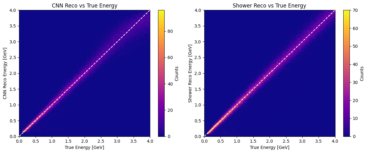
# lets evaluate with test dataset and compare to the showerE (conventional method)

recoE, thrownE, showerE = evaluate(model, test_loader, desc="Testing", returnShowerE = True)

import matplotlib.pyplot as plt

MIN_E = 0.0
MAX_E = 4.0
BINS = 200

plt.figure(figsize=(12,5))
plt.subplot(1,2,1)
plt.hist2d(thrownE, recoE, bins=BINS, range=[[MIN_E, MAX_E], [MIN_E, MAX_E]], cmap="plasma")
plt.plot([MIN_E, MAX_E], [MIN_E, MAX_E], "w--")
plt.colorbar(label="Counts")
plt.xlabel("True Energy [GeV]")
plt.ylabel("CNN Reco Energy [GeV]")
plt.title("CNN Reco vs True Energy")
plt.subplot(1,2,2)
plt.hist2d(thrownE, showerE, bins=BINS, range=[[MIN_E, MAX_E], [MIN_E, MAX_E]], cmap="plasma")
plt.plot([MIN_E, MAX_E], [MIN_E, MAX_E], "w--")
plt.colorbar(label="Counts")
plt.xlabel("True Energy [GeV]")
plt.ylabel("Shower Reco Energy [GeV]")
plt.title("Shower Reco vs True Energy")
plt.tight_layout()
plt.show()

import numpy as np
import matplotlib.pyplot as plt

# ----------------------------
# Parameters and binning
# ----------------------------
bins = np.arange(0.1, 4.0 + 0.25, 0.25)
bin_centers = 0.5 * (bins[1:] + bins[:-1])

# ----------------------------
# Function to compute sigma + plot histograms
# ----------------------------
def compute_and_plot(thrownE, testE, bins, label="recoE"):
    res_sigma, res_err, res_data = [], [], []

    for i in range(len(bins) - 1):
        mask = (thrownE >= bins[i]) & (thrownE < bins[i+1])
        if np.sum(mask) < 10:
            res_sigma.append(np.nan)
            res_err.append(np.nan)
            res_data.append(np.array([]))
            continue

        ratio = (testE[mask] - thrownE[mask]) / thrownE[mask]
        sigma = np.std(ratio)
        err = sigma / np.sqrt(2 * len(ratio))  # rough error estimate

        res_sigma.append(sigma)
        res_err.append(err)
        res_data.append(ratio)

    # ----------------------------
    # Plot subfigures of distributions
    # ----------------------------
    ncols = 5
    nrows = int(np.ceil(len(bins) / ncols))
    fig, axes = plt.subplots(nrows, ncols, figsize=(20, 3*nrows), sharey=True)
    axes = axes.flatten()

    for i in range(len(bins)-1):
        ax = axes[i]
        data = res_data[i]
        if len(data) == 0:
            ax.axis("off")
            continue

        ax.hist(data, bins=30, histtype='stepfilled', alpha=0.6, color='C0')
        ax.axvline(0, color='k', linestyle='--', alpha=0.5)
        ax.set_xlim(-1, 1)
        ax.set_title(
            f"{bins[i]:.2f}-{bins[i+1]:.2f} GeV\n"
            f"σ={res_sigma[i]:.3f} ± {res_err[i]:.3f}",
            fontsize=10
        )
        if i % ncols == 0:
            ax.set_ylabel('Counts')

    for j in range(len(bins)-1, len(axes)):
        axes[j].axis('off')

    fig.suptitle(f"Relative Energy Residuals per ThrownE Bin ({label})", fontsize=14)
    fig.tight_layout(rect=[0, 0, 1, 0.96])
    plt.show()

    return np.array(res_sigma), np.array(res_err)


# ----------------------------
# Compute and visualize
# ----------------------------
sigma_reco, err_reco = compute_and_plot(thrownE, recoE, bins, label="CNN RecoE")
sigma_shwr, err_shwr = compute_and_plot(thrownE, showerE, bins, label="Conventional ShowerE")

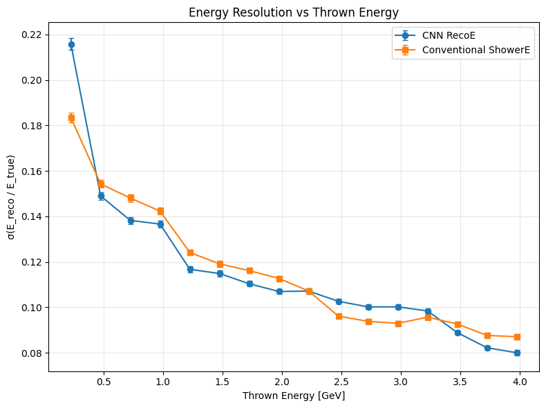
plt.figure(figsize=(8,6))
plt.errorbar(bin_centers, sigma_reco, yerr=err_reco, fmt='o-', label='CNN RecoE', capsize=3)
plt.errorbar(bin_centers, sigma_shwr, yerr=err_shwr, fmt='s-', label='Conventional ShowerE', capsize=3)

plt.xlabel('Thrown Energy [GeV]')
plt.ylabel('σ(E_reco / E_true)')
plt.title('Energy Resolution vs Thrown Energy')
plt.grid(True, alpha=0.3)
plt.legend()
plt.tight_layout()
plt.show()

Exercise to Try Out

Now that we have successfully regressed the shower energy using the CNN model, you can take it a step further and test its impact on physics reconstruction.

🧩 Task Overview

Replace the conventional showerE with the CNN-regressed energy (recoE) in the physics reaction reconstruction chain.
For example, in the ω → π⁺π⁻π⁰ → π⁺π⁻γγ channel, substitute the neutral shower energies with the regressed ones and observe the change in the reconstructed ω invariant mass distribution.

🧪 Goal

Check whether using the CNN-predicted energies leads to a narrower ω mass peak, indicating an improvement in energy resolution and hence better physics fidelity.

⚙️ Suggested Pipeline

1. Photon Selection

   • Identify neutral showers in each event.

   • Use the trained CNN classifier to check if a neutral shower is a good photon candidate (i.e., not a hadronic splitoff).

2. Energy Regression

   • For the showers classified as good photons, replace the conventional showerE with the CNN-regressed energy (recoE).

3. Physics Reconstruction

   • Reconstruct the π⁰ candidates and ω candidates using the new energies.

   • Compare the resulting invariant mass spectra with the baseline (using showerE).

4. Resolution Study

   • Quantify the improvement by fitting the ω mass distribution with a Gaussian (and possible background function).

   • Compare σ(ω) between the two cases.

🔍 Further Explorations

• Perform a more detailed fit to the energy resolution curves, The energy resolutions it self can be fit with appropriate curves to extract the resolution in each bin. Followed by a fit to the energy resolution curves e.g. using a calorimeter-like parameterization: $\( \frac{\sigma_E}{E} = \frac{a}{\sqrt{E}} \oplus b \)$ and study how tuning the CNN architecture or training data affects the stochastic and constant terms.

• Investigate how different noise levels or thresholds in the FCAL hit patterns influence the regression accuracy.

• Try propagating the energy uncertainty from the regression model into the invariant mass reconstruction and study how the uncertainty on σ(ω) evolves.